When I did Physics at University I was taught that the world was deterministic, that F=Ma was not an approximation, but what actually occurred and that any deviation from this was merely an inability to measure precisely enough. This was a concept so ingrained into the philosophy of science that it was only by doing a course on philosophy that I was made aware of this philosophical deterministic viewpoint of science.
Then in my final years I also did electronics, in which I was taught my first formal concept of noise. Finally I went into engineering, where almost everything is noise and the skill is to find the small part of the real world which can be measured and predicted deterministically using scientific principles.
But looking at science now I realise that it has far more models of “noise” than I had imagined. In other words, various subjects have adopted ways to reconcile the real world which is full of noise and variation with the idealistic deterministic world taught in science. In short, I will show that whilst the philosophy of science is that the world is deterministic – that everything is predictable – in reality even science has to compromise with various fudges and fixes to cope with the real world which is not deterministic.
First a definition of “formal noise model”:
A model, formula or other construct that formally defines the known behaviour of a system which also includes unknown behaviours which are “hidden” (ignored?) behind the formal noise model.
Now I will briefly outline the concept of noise as most scientists are taught it.
“Scientific” Noise
As I said above, the philosophy of science is that underlying the universe is a deterministic set of rules such as “F=Ma”. If we carry out an experiments and we find that the force does not equal the mass times acceleration, then the philosophy of science says that because the rule is a “law” the reason for the deviation is that there has been “measurement error”. Note the terminology: “error”. This implies there is a correct value from our deterministic law and pesky equipment is stopping us seeing it because the equipment is introducing “false” perturbations preventing us measuring the “correct” value. (compare this to quantum mechanics below)
Most scientists are only taught one kind of measurement error: this is a small perturbation of the signal due to many unknown factors which has two properties:
- It is a Gaussian (in reality it only approximates to one)
- Implicitly that the noise is “white noise” which has the convenient property that the error decreases as √n where n is the number of samples.
Gaussian noise is an approximation to the probability distribution obtained if a large number of small, random and uncorrelated events occur. White noise has the advantage that an improved measurement can be obtained by merely repeating the experiment. So by taking four times as many results, the “error” can be reduced by half.
It also has the advantage that the noise power is additive (if two measurements with Gaussian noise are multiplied then the square of the final “error” is sum of the squares of the individual error). But this is only true if the causes of error in each of the values is unrelated and that their values are uncorrelated – however this is usually true in simple laboratory experiments (this correlation is not dealt with further in this article).
The model of this noise is as follows that for an input x output y and a physical law f() then noise is seen as fitting the following (where n is number of times experiment repeated):
y = f(x) + Δ
(where Δ → 0 as n → ∞)
so that for a system with “scientific noise”, in order to obtain an acceptable “error”, the experiment can be repeated, or a larger data set obtained until the error is below the required size. Thus for all reasonable purposes the relationship can be expressed excluding any error term as:
y = f(x)
And because of this property of white or perhaps it might be called: “scientific noise” that the world can be considered deterministic and if only enough funds were available all unwanted variation can be removed by simply obtaining more and more data. In other words it is the view that:
a scientist looks at the signal in data, not the noise.
The above view, is however false. In the real world, noise, natural variation and other unwanted perturbations (including human) exist which cannot be removed and there are various ways to deal with them, both in engineering and science.
“Scientific” Noise with input noise
Where a system is subject to an input signal whose value is subject to “instrumentation error”, Δin the model of “scientific noise” says that the output from an experiment with a transfer function f(x) and reading error Δout is:
y = f(x+ Δin) + Δout
Simple Electronic Noise
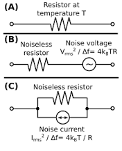 One of the simplest noise models is that shown to the right. Top is shown a simple resistor. It has a theoretical relationship to voltage and current as follows:
V = IR
However, in real life the resistor does not follow this rule, but instead there is a noise value from the resistor due to a number of factors: the discrete nature of voltage due to the potential of each electron; the discrete nature of charge, due to the charge of each electronic, and ongoing degradation and changes in the resistive material so that there are steps up & down in the conductance of channels through the resistive material.
In order to model this noise, various models are used of which the most common two are shown above. The first is to introduce a potential energy source which has zero resistance and develops a potential difference across itself as follows (assuming only discrete noise sources):
vn = √(4kBTRΔf)
where
vn is the noise potential difference across the resistor
kB is the Bolzman constant in joules per Kelvin (1.3806488(13)×10−23)
T is temperature in Kelvin
R is resistance in Ohms
Δf is the bandwidth in hertz over which the noise is measured.
The second is a noise current source which is as above except it has infinite resistance and voltage and potential are related by vn = in R
Fundamental change
Whilst electronic noise and “scientific noise” may look the same, there is now a fundamental change in philosophy which is apparent in the names given. In science, the name for variations tends to be “instrument error” – something external to the theoretical construct. Whereas this new eletronic model is called “resistor noise” – something attached to a component within a circuit. It is now treated like any other deterministic potential – except its precise value is unknown at any one time. Like “scientific noise”, which tends to zero as more and more measurements are taken, because Δf = 1 / ΔP (where ΔP is the period or length of measurement), if more and more measurements are taken
(vn → 0 as ΔB → ∞)
So for a large period/dataset it appears that this electronic noise models are the same model as “scientific noise” as:
V=IR + vn
(vn → 0 as ΔB → ∞)
so at ΔB = ∞
V=IR
However, the main reason for this noise model, is not in steady state systems, but in real life circuits such as audio amplifiers where there is a finite bandwidth. ΔB cannot go to ∞ and as a result noise can never be eliminated. In other words, it is always present, so it is not true that vn→0
This is why electronic noise is treated fundamentally differently from “instrumentation error”. This is because the noise as in the climate is always part of the system.
1/f (flicker) type Electronic Noise
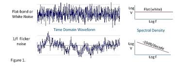 1/f or more accurately f-n or indeed, realistically frequency dependant noise: F(f) noise, is noise whose power per bandwidth changes dramatically with frequency. The result is that it is rich in low frequencies, so that unlike “scientific noise” shown top which “dances” like an energetic disco-dancer rooted to the spot in a crowded club, flicker noise tends to go wondering with long excursions rather like a free waltz in ballroom dance.
And whilst few scientists get taught the theoretical nature of flicker noise so it appears to be unusual, such noise appears to be ubiquitous and it is only in some special instances whereby normal frequency dependant noise can be approximated by white or “scientific noise”.
Those lecturing students – particularly those from a science background – on 1/f noise must have fun when they first state the frequency relationship of 1/f noise. Because unlike white noise where the noise per unit bandwidth is constant, the noise per unit bandwidth at a frequency f is given by:
vn ∝ 1/f
Whereupon the brightest ones, (should) say “but that is not possible as at zero hertz there’s infinite noise”.
Unfortunately (at least when I was taught) this isn’t taken as an opportunity to go into the theoretical nature of 1/f noise and instead (we went) into its practical implications: that in a system where 1/f noise dominates, that the usual practice of taking more and more readings doesn’t work, and various practical ways are suggested to get around the problem.
If I remember correctly, this was then used to explain the need for “chopper circuits” – so perhaps this will help. The reason for this, is many semiconductors suffer from 1/f noise in the sensitive input circuitry. This means that if a very precise measurement needs to be taken, 1/f noise (seen as a drift in the input voltage/current) adds randomly to the input severely limiting the accuracy. A way to eliminate this, is to invert the input at a specified frequency, amplify it and then invert it again after amplification. If the inversion mechanism is very low noise this results in an average output from an input v (inverted periodically to -v) of
Vout = A.(v + vn)/2 + -A.(-v + vn)/2
Vout = A.v + A. (vn/2 – vn/2)
Vout = A.v
What is actually happening, is that the chopper circuit changes the frequency of the input. So that if the chopper is 1000Hz, then an input signal varying at a very slow frequency of say 0.01Hz whose noise would be proportional to 1/0.01Hz so large, is converted to a frequency at 1000 ±0.01. This means the amplifier is working with a frequency of 1000Hz and not 0.01Hz and the resultant noise at 1000Hz is proportional to 1/ (1000 ±0.01) or around 1/100,000th of that of a non-chopper circuit.
Climatic modelling – Ensemble forecasts
Whilst I have looked (notably Tim Palmer Predictability of weather and climate), I have found no climatic model that includes any formal concept of noise or natural variation. Instead natural variation only seems to be catered for by ensemble forecasting. This is a reformulation of “scientific noise” (ignoring output noise):
T = f(t+ Δ)
where
T – is output (assumed temperature)
f – is function of model
t – are input parameters
Δ – are perturbations to input parameters
Hence, it is believed that climatic variation can be modelled by an “ensemble” of forecasts by perturbing input parameters so that a number of forecasts are produced:
T1 = f(t+ Δ1)
T2 = f(t+ Δ2)
…
Tn = f(t+ Δn)
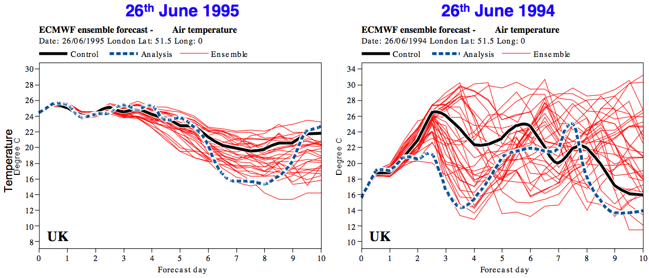
Source: http://www.easterbrook.ca/steve/2010/07/tracking-down-the-uncertainties-in-weather-and-climate-prediction/
The kind of result produced from this analysis is an ensemble forecast as above. Each line represents one model run using one set of perturbations. The assumption is that by trying a range of perturbations, these are likely to include all future states of the system and that the probability of any state is proportional to the number of perturbed model runs that have that forecast value.
The Failure of Initial Parameter Perturbation
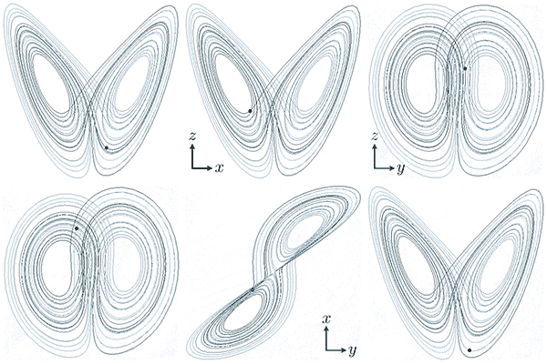 The problem is best illustrated with a Lorentz “butterfly”:
This shows the “path” taken by a formula by successive applications of the formula. Whereas we might expect the result to be chaotic, the importance of the Lorentz butterfly is that it reveals order in disorder. Thus in the butterfly, the order is shown by the way the function occupies a defined region and how, whilst the long term value is chaotic and thus impossible to predict, in the short term, the function “moves” along very predictable curves, within the very predictable space.
Moreover, just as Lorentz did not predict this order, so this “predictability” is difficult to “predict” in other systems. So it may (or perhaps always) exists in climate models.
We can generalise this as follows:
- Complex systems are both predictable and usually unpredictable in their long-term behaviour
- Small changes in initial conditions can result in very large differences in long term state.
- Large changes in initial condition can be constrained in unforeseen ways so that the final state is closer together than expected.
These constraints tend to limit the variation within the system. In a sense we should see “variation” as a property of the system which tends to decay by being constrained.
To give a simple example, imagine a model used to predict crowd behaviour. Each person is modelled as leaving home for a football match. The route to the fixture is a walk to a train station, then a walk to the football match.
In order to model “variability” in this system (like the ensemble forecast) we introduce a different time for them to leave their house. They all leave the house – whereupon they all go to their individual stations – where they all wait for the same train – which because there is no variability for the train arrival in the model – they all board as it arrives. But this means (ignoring late comers) they board it at the same time irrespective of when they leave the house. Therefore, from this point onward variability has been removed. Because when they leave the train (arriving at fixed time), their exit time from the train is determined not by the variable time they left the house, but when the train arrives – which does not vary.
Thus, because the model is constrained by an internal “choke” point, this tends to remove the variability in the initial perturbation. The result is that the “scale” of variability or “noise power” is severely reduced by internal constraints within the model.
How then, do we model such a system? The answer, is simple: we must re-introduce variability as the model runs. Thus, Instead of having the participants leave ±10minutes at the start as “initial perturbation” (which we assume is enough to catch the train), we could have them leave ±1min, then have then take ±1min to exit the train. ±1min to reach the entrance, then ±1min to get through the entrance queue, etc. totalling in sum ±10min.
Perversely, this is starting to behave like “scientific noise” – that is instead of one big perturbation as we find in initial value perturbation, we instead have a lot of small changes that add together. We could then keep adding in new forms of perturbations – changes to walking speed, random delays – queues going into the train displacing the traveller so that this in turn changes their arrival time. The more we have the more it resembles “Gaussian” noise. But most importantly, the “noise power” must not be allowed to disappear through “constraints” in the system, which is what happens with initial value perturbation.
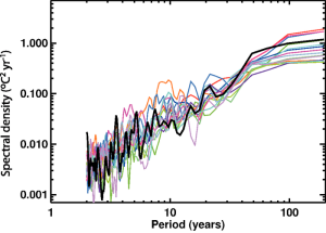
Fig 1: Variability of observed global mean temperature as a function of time-scale (°C2 yr–1)
from figure 9.7 IPCC (2007)
Statistics of 1/f noise
First, looking to the right, we can see the variability observed in the global temperature signal and that it varies linearly on this log scale with period, increasing as the period lengthens (as frequency decreases). And we can readily see this is 1/f type noise as at an infinite period (zero frequency), the scale of variation will be infinite
Very little has been written about the statistics of 1/f noise. In my view (and some papers I’ve read) this is because there is no real understanding of how 1/f or flicker noise is produced. Indeed, it may derive from very different processes that just happen to produce the same frequency dependent noise profile. So the following statements are hedged with “this appears to be true”. Within the same signal, these are the basic rules:
More data points mean more noise
This is the most confusion aspect of 1/f noise – that as the period of measurement increases, so the minimum frequency present in the sample tends to decrease. And because noise increases as 1/f as f→0 so noise→∞.
To compare the two as we obtain more samples
Flicker noise (as samples→∞ f→0)
noise/signal→∞
white noise (as samples→∞ f→0)
noise/signal →0
Thus when flicker noise is present, rather than improving with more samples, equipment deteriorates. Usually this is separated out and seen as “requiring calibration” rather than being a type of noise. That is to say, the equipment has “drifted”, which is treated as a distinctly different behaviour to usual “scientific noise”. However, in real systems there are usually (always?) several types of noise each with their own frequency profile, so in a theoretical model of noise of systems which are used for extended periods their noise model must include the 1/f noise.
And when we start talking about climate over centuries and millennium, 1/f noise will certainly be present (as noise increases over longer periods). The result, is that far from reducing “natural variation” through extended sample periods, the result of increased sample periods is to increase the natural variation present – which can all too easily be seen as a “signal” (see: Natural habitats of 1/f noise errors.)
Statistical tests must be based on equal periods
I’ve already mentioned above how “chopper” circuits can be used to largely remove 1/f noise. In another form, this strategy can be used to get around the problem with long term noise. The problem with a system like the climate is that the noise and signal have very much the same rates of change (same frequencies). So it is not possible to use any techniques like averaging which are really forms of low pass filter – intended to filter out the low “signal” frequencies from the high frequencies in “scientific noise”.
So, e.g. we regularly see around 0.1C/decade change due to natural variation in the Central England Temperature record. But the temperature of the globe warmed around 0.8C over the last century. How can we distinguish between noise and signal when they are so similar?
One way to do this is to assess a very long period without the signal and then to characterise the noise and then compare the period under examination with the “null hypothesis” of this “natural variation”. However, when we only have a short period like the global temperature, this is clearly not possible. However, whilst we do not know the noise profile without a long period, what we do know, is that equal periods allow the same frequencies, so the scale of noise should be similar. Thus the best** we can do with a short time run, is to compare like periods. This is what I did here.
**A more complex analysis would be possible – but it would not greatly improve the result.
What goes up doesn’t necessarily come down
I’ve been running the experiment on 1/f noise at uburns.com which illustrates a rather quirky behaviour of 1/f noise (or at least the 1/f noise generator I use). Below is a plot of the trend in the final 1/16 of the run against the value (simulated temperature).
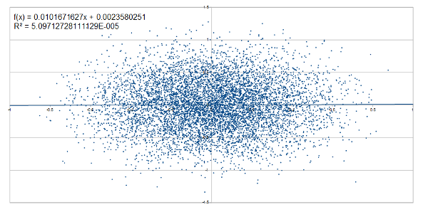 We naturally tend to think that things that go “high” will tend to come back to “normal”. Or in the case of “natural variation” that a departure from normality that will (eventually) be restored at some point. However, if this were true, then values to the right which are high, would tend to have a positive trend to tend to bring them back to zero, and those to the left (low) would tend to have a negative trend to bring them back down.
But this graph with a R2 value of 0.00005, shows that using the 1/f generator I have that the trend when the “temperature” is high is not in any way biased toward cooling. Neither when the plot it cooler, is it biased to warming. So, it never “tends toward zero”.
In layman’s terms: “what goes up … doesn’t know it shouldn’t be up”. If this is how the climate behaves, then it suggests that if we see 1C warming – then the best estimate of future temperature (if there is nothing but natural variation) is that it will remain 1C warmer … although there is an equal probability that it will get warmer or cooler than 1C … it’s just that 1C warmer is the best estimate of future temperature.
Formal Noise models
I have already covered various “noise models”:
- “Scientific noise” or “instrumentation error”
- “Scientific noise” with initial value “instrumentation errors”
- Simple Electronic noise (gaussian white noise)
- 1/f (flicker) noise
- Ensemble forecasting
Now however I wish to illustrate some other formal noise models in science:
- Hydrological
- Quantum probability wave
- Thermodynamic
- Evolution
Hydrological
This is a very simple model, which says that river probability of river flow (y) follows a Gaussian distribution** when plotted by the log of flow (x). This is a formula found to be generally applicable to most rivers and predicts the probability of any flow level. What it means is that most of the time the river flow is relatively low (well within the banks), but that quite “normally” it will flow high, and quite often (once a year) it will tend to overflow the banks with perhaps 100x the “normal” flow. These flow charts are used to determine the likelihood of a serious flood event even when no such flood event has been recorded in the records.
The importance of this model for climate, is that it shows that whilst individual contributions from rainfall, may be “random”, the net effect because of correlation between events in a region (as rain tends to fall in a region), is that these small “raindrops” can build to an almighty “flood” of variation. Thus the sum total of small “scientific noise” like changes from each raindrop is not random, but because of geological and physical features, it follows a very specific “noise model” for river systems.
However, as evaporation from the earth’s surface is a substantial proportion of heat transfer – because evaporation is driven by rain in an area, because rain and river flow are linked, then the same factors affecting river flow variation will be present (at least to some extent) in climate variation.
A deterministic model of climate must either model each and every raindrop – a totally impossible task – or it must model all the potential regional variations of climate due to rain – which again is impractical – or like the resistance model of noise – it could adopt a formal noise model akin to the “noise source” in electronics which acts to constantly introduce variation into the system.
**This is often modified to include a skew parameter.
Quantum probability wave
One way of viewing a probability wave (not recommended), is that a “photon” exists as a particle, but that’s its position (& energy) is unknown. Put this way, it shares similar properties to the hydrological model: a simple probability function. And likewise that probability function can be used to predict behaviour.
However, usually the “wave” is seen as a facet of the photon itself. How it exists is a matter of philosophical debate, but its practical use cannot be denied because the probability of interaction with matter can be predicted from this model. This model predicts “it” behaves like a “wave” showing diffraction and refraction patterns.
As such, practically, it is a way to describe unknown variations within the physical world in a predictable way. It is a formal “noise model” – describing “natural variation” of a photon whose behaviour cannot be known because the initial conditions of the photon cannot be known. So, by creating a formal model, the behaviour of the system can be predicted, not by knowing the initial conditions, but by the way the “noise model” or “probability wave” behaves.
Thermodynamics
Thermodynamics (at least here) is fundamentally the statistics of random movement between particles. According to the deterministic philosophy of science, the movement of particles can be predicted absolutely. But according to the Lorentzian world where small changes grow in significance, it cannot. Moreover, there is a fundamental limit based on quantum mechanics to how much we can know about a system built of particles of finite size.
Thus, whether we like it or not, the initial state of complex many-particle systems cannot be known with enough knowledge to predict their behaviour even over a limited number of collisions and certainly the behaviour or any one atom in terms of speed position and energy cannot be predicted over the long term.
Thus, in Thermodynamics there is a formal model of “noise” called “heat”. Like quantum mechanics and hydrology, there is a probability distribution that describes the probability of finding an atom with a certain energy. This probability model can then be used to predict the behave of a large ensemble to external forcings such as pressure or temperature.
To go back to the climate analogy – if “initial perturbations” were used in thermodynamics, then this would involve slightly changing the speed and position of all atoms. But like the Lorentz type calculations which show massive changes to small changes to the computer code, as well as “strange attractors” – given the huge numbers of calculations to model even a few atoms over an extended period, there is little doubt that the form of calculation would have a profound effect on the way the model behaves . E.g. we could end up with oscillations or some similar effect due to peculiarities of the way the code interact. These will not be present using a simple macro-scale models of “heat”.
However, by moving to a model of “heat”, we no longer have a deterministic system. In other words heat creates a way to have a formal model of “noise” within the movement of atoms. The scale of that movement then relates to temperature.
And because there is a form model of “noise” or natural variation within Thermodynamics, usually thermodynamic systems can be analysed without even considering the deterministic processes being applied to individual particles.
However, should we look at very small particles like “smoke” or processes like diffusion – we do have to go back and model the individual, and within the context of heat, random behaviour of particles.
Evolution
So far I have examined systems where there is a formal model of “noise” which is largely predictable. However, now I would like to show that formal models of noise, or in this case “natural variation”, have utility in science even when their exact form and value are unknown.
Natural variation is a concept in evolution stating that individuals vary from each other “naturally”. At the time of Darwin, there was little understanding how this natural variation could exist. But even though it described a concept of “noise” within the characteristics of animal populations and even though there was no idea how it was created nor what “scale” it took, there is no doubt whatsoever that it was a critical part of the theory of evolution.
And to go back to the idea that systems can be modelled using “initial perturbation”. If applied to the evolution of animals, this would imply that e.g. 100 fish pulled themselves out onto the mud. One of them would have been “most fit” – and thus if you believe the idea that systems can be modelled with “initial perturbation” – you are in effect claiming to be a clone of that fish!!
Because, natural variation does not work unless more variation is introduced into each and every generation. So whilst “natural selection” tends to weed out weaker traits, “natural variation” constantly occurs to maintain a diverse population.
This is what is missing in the climate models – there is no way to maintain that natural variation in the system – indeed, I do not believer there is any concept within climate models of formalising “noise” or “natural variation” – so there is nothing to be “maintained” because it is not part of the model in any shape or form.
Addendum – Autoregressive model
Just for clarification, “flicker noise” is often treated in statistics using an Autogressive model. The autoregressive model specifies that the output variable depends linearly on its own previous values and on a stochastic term (a stochastic meaning an imperfectly predictable term or “noise”).
These are generally described as follows:
![]()
Where Xt is the output at point t, c is a constant, φp are the parameters of the model, and εt is Gaussian white noise. For simple systems where the output is the current input plus a a single contribution being a constant times the last output thee frequency profile can be calculated:
![]()
where σe is the standard deviation of εt.
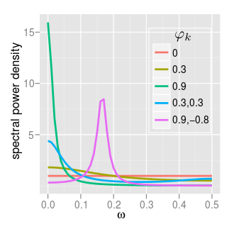
This gives various frequency responses as shown right. Using a complex series of parameters, various frequency responses can be approximated. Thus with enough parameters, various types of 1/f or flicker noise can be modelled using techniques that are easier to analyse statistically.


Interesting, SS. I spent a bit of time a while ago playing with analogue/digital converters, Nyquist, Fourier and all that good stuff.
The other thing that the climate “scientists” never seem to incorporate any appreciation of entropy.
As a chemical engineer, entropy came into everything, I couldn’t tale a leak without considering entropy/enthalpy relationships.
I suppose entropy’s like noise, far, far too complicated for climate “scientists”.
That’s “take a leak”, of course!
Their argument is thus: the climate is constrained – we know what is coming in and out – there’s nothing to drive “natural variation”.
The counter argument is thus: even a f*ing resistor has noise – you must be b** insane to think that if a small resistor has noise, then something as big as the planet will not.
Of course, their position is totally illogical. They claim “natural variation” – can all be attributed to known effects – of which the largest is CO2. But as natural variation is shown throughout CET and does not change in scale, this means that if CO2 were driving natural variation now, it would have been the predominant AND NATURAL cause of variation throughout CET.
This is why they will never ever talk about CET – because it proves they are just making up human attribution.
Pingback: Judith Curry: Natural variability – does she get it? | Scottish Sceptic
Klimushkin M., Obiedkov S., Roth C. (2010) Approaches to the Selection of Relevant Concepts in the Case of Noisy Data. In: Kwuida L., Sertkaya B. (eds) Formal Concept Analysis. ICFCA 2010. Lecture Notes in Computer Science, vol 5986. Springer, Berlin, Heidelberg
By the way! The best essay writing service – https://www.easyessay.pro/
And Happy New Year!