I spent a few days this week creating a greenhouse gas model of the atmosphere – originally intended to show that the greenhouse effect on the various planets can easily be explained using fairly straightforward physics.
Initially, I created a model based on a single greenhouse gas molecule which acted uniformly across the IR band and with no clouds. I didn’t have figures of the scale of IR absorption I should use, so I simply put in a fudge factor to bring the greenhouse effect to 33C.
However, when for interest I looked at the effect of doubling this greenhouse gas concentration, I got a massive response (perhaps 4C/doubling). So, for interest I then added a second greenhouse gas which was modelled as if the two gases were equal in effect, but one (assumed CO2) absorbed in one fraction of the spectrum and the other in the remaining part (assumed to be H2O). However, when I tried to tune the effect to get the required 1C/doubling of CO2, I found I needed to reduce the band occupied by CO2 to 4% which was quite ridiculous. It appeared I was making a simple arithmetic error somewhere but I just could not find it.
So, next I decided to use actual gas constants for CO2 and H2O. But that suggested the figure I was using was about 1/100 of the actual value. So, finally I tried to model the actual concentrations of water vapour in the atmosphere.
 
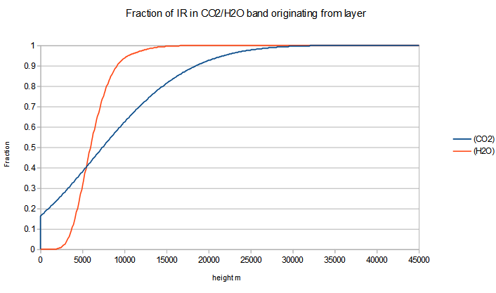
Only when I added this second greenhouse gas could I get anything near the typical figures used for gas typical absorption coefficients (and I had to work these out myself using tables and planck laws). However the kind of result I get is as follows. For simplicity I plot the percentage of radiation leaving the planet from each layer for the two greenhouse gases I have. (note this also has a 10% “cloud effect” – which is treated as a raised surface of fixed temperature at a cloud height covering 10% of the “window”).
There are still large errors in this graph – probably because the model and atmosphere are very sensitive to “masking effects” whereby each additional complexity – such as adding clouds, seems to reduce the fudge factor I need and in turn reduces the impact of CO2. So, the current model gives a greenhouse effect of doubling CO2 of 2C – but with a “fudge factor” of ~0.5.
What this means is that in order to get a greenhouse effect of around 33C, I have to scale down the absorption coefficients by 50%, but because probably because the effect of doubling CO2 has a logarithmic impact the effect of a doubling of CO2 has the same impact and so remains twice as high even when the total greenhouse effect is scaled down appropriately.
In other words, the models are extremely sensitive to the assumptions made about which greenhouse gases and how their frequencies overlap.
And, perversely, whereas I would intuitively have thought that a less complex model with less elements would tend to underestimate the greenhouse effect, I’m finding in practice that the simplest models tend to over-estimate the sensitivity of elements like CO2. And thus the more complex the model, it would seem the lower the CO2 sensitivity would become.
The obvious missing element are clouds & “band masking”. And e.g. I couldn’t hope to model the greenhouse effect on Venus if I did not take account of the massive layer of clouds in its atmosphere.
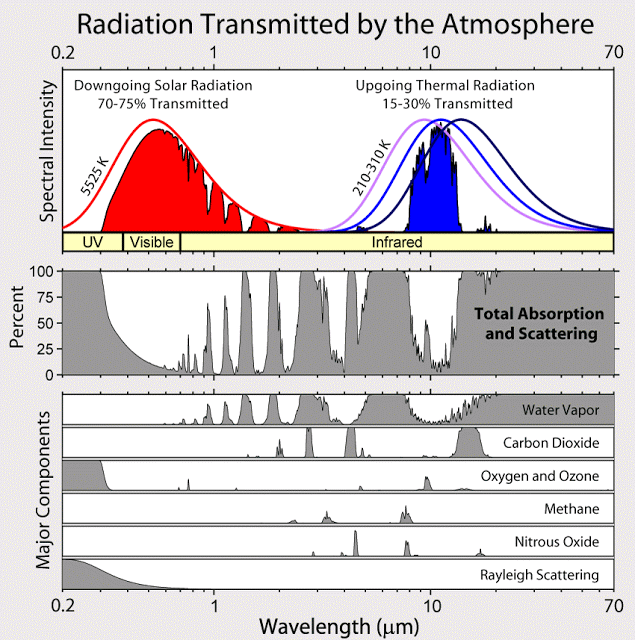
But band masking is a serious problem for me (and indeed anyone doing modelling), because CO2 absorbs in the same spectral region that water vapour is active as seen below. As you can see water vapour absorbs around half the frequencies between 10-20um where CO2 has its absorption band in the infra-red. (Which might equate to my 0.5 fudge factor, but I’ve made similar assumptions with the model before and been wrong). And it was precisely because of this “band masking” (but in a much more complex form) that Hermann Harde calculated a much smaller climate sensitivity.
To model the CO2/H2O I started by treating CO2 as being exclusively dominant in a narrow band of the IR (16% 13.235 – 16.660um). Then to get a more sensible greenhouse sensitivity I added water vapour as being dominant in its own “band”. (77%) Unforunately, the absorption data I am using gives no data for H2O in the CO2 band, but the above graph says otherwise. I could guess the effect, but should I just replace one fudge factor with another?
The cloud effect is more complex – because water droplets behave very different optically to water vapour but for obvious reasons water droplet and water vapour are active in the same spectral regions so I need an even more complex model. I could model tropospheric cloud as if it were water vapour, the effect would be to show a “jump” in the fraction of IR from water in the top graph at the tropospheric cloud layer (and the curve below would be adjusted to show less effect from H2O). However, if I add tropospheric cloud, I then feel I ought to add stratospheric cloud – but as the graph shows, I currently have almost no impact from H2O at 20km, the typical height of stratospheric cloud formations.
With a bit of thought I think I could easily add in earth’s clouds – but then how do I translate this to other planets what does “stratospheric cloud” mean on Venus, Mars or Triton? The more complexity I add to the model to represent what is happening in our atmosphere, the less general it becomes and the less it fulfils the original purpose of modelling all atmospheres.

Conclusions of exercise

Firstly I am very surprised that how sensitive the model is to the initial assumptions I make. That is to say, rather than starting reasonably close and getting closer & closer as I add in more detail. The model seemed to “bounce around” giving relatively large changes for small changes in my assumptions and even a fairly complex model still needs a massive 50% fudge factor.
Secondly, some of the behaviour is counter-intuitive. Particularly the way adding in more greenhouse gases & more components seem to reduce the overall sensitivity (CO2 operates relatively high so is least like the ground whilst other components are lower so are closer to the ground temperature).
Third, the overlapping spectrums both in terms of frequency as well as their differing effects with height is a major headache in the model.
Fourth, whilst I’ve used a single “1D” atmosphere – which is a good representation of a well mixed gas like CO2, H2O is not well mixed and there are significant changes in e.g. water vapour concentrations between the equatorial regions and polar regions. There’s also as much as a 40C difference in surface temperature. The ground surface temperature is relatively unimportant, but the differing tropospheric height and water vapour profile will undoubtedly significantly affect the greenhouse effect.